Monte Carlo...again
A Monte Carlo method is a technique that uses random numbers and probability to solve complex problems. The Monte Carlo simulation, or probability simulation, is a technique used to understand the impact of risk and uncertainty in financial sectors, project management, costs, and other forecasting machine learning models.
Risk analysis is part of almost every decision we make, as we constantly face uncertainty, ambiguity, and variability in our lives. Moreover, even though we have unprecedented access to information, we cannot accurately predict the future.
The Monte Carlo simulation allows us to see all the possible outcomes of our decisions and assess risk impact, in consequence allowing better decision making under uncertainty.
Example - Roll the dice
Our simple game will involve two six-sided dice. In order to win, the player needs to roll the same number on both dice. A six-sided die has six possible outcomes (1, 2, 3, 4, 5, and 6). With two dice, there is now 36 possible outcomes (1 and 1, 1 and 2, 1 and 3, etc., or 6 x 6 = 36 possibilities). In this game, the house has more opportunities to win (30 outcomes vs. the player’s 6 outcomes), meaning the house has the quite the advantage.
Let’s say our player starts with a balance of $1,000 and is prepared to lose it all, so they bet 1 on every roll (meaning both dice are rolled) and decide to play 1,000 rolls. Because the house is so generous, they offer to payout 4 times the player’s bet when the player wins. For example, if the player wins the first roll, their balance increases by 4, and they end the round with a balance of 1,004. If they miraculously went on a 1,000 roll win-streak, they could go home with 5,000. If they lost every round, they could go home with nothing. Not a bad risk-reward ratio… or maybe it is.
We can define a function that will randomize an integer from 1 to 6 for both dice (simulating a roll). The function will also compare the two dice to see if they are the same. The function will return a Boolean variable, same_num, to store if the rolls are the same or not. We will use this value later to determine actions in our code.
# Creating Roll Dice Function
def roll_dice():
    die_1 = random.randint(1, 6)
    die_2 = random.randint(1, 6)
    # Determining if the dice are the same number
    if die_1 == die_2:
        same_num = True
    else:
        same_num = False
    return same_num
Every Monte Carlo simulation will require you to know what your inputs are and what information you are looking to obtain. We already defined what our inputs are when we described the game. We said our number of rolls per game is 1,000, and the amount the player will be betting each roll is $1. In addition to our input variables, we need to define how many times we want to simulate the game. We can use the num_simulations variable as our Monte Carlo simulation count. The higher we make this number, the more accurate the predicted probability is to its true value.
The number of variables we can track usually scales with the complexity of a project, so nailing down what you want information on is important. For this example, we will track the win probability (wins per game divided by the total number of rolls) and ending balance for each simulation (or game). These are initialized as lists and will be updated at the end of each game.
# Tracking
win_probability = []
end_balance = []
In the code below, we have an outer for loop that iterates through our pre-defined number of simulations (10,000 simulations) and a nested while loop that runs each game (1,000 rolls). Before we start each while loop, we initialize the player’s balance as $1,000 (as a list for plotting purposes) and a count for rolls and wins.
Our while loop will simulate the game for 1,000 rolls. Inside this loop, we roll the dice and use the Boolean variable returned from roll_dice() to determine the outcome. If the dice are the same number, we add 4 times the bet to the balance list and add a win to the win count. If the dice are different, we subtract the bet from the balance list. At the end of each roll, we add a count to our num_rolls list.
Once the number of rolls hits 1,000, we can calculate the player’s win probability as the number of wins divided by the total number of rolls. We can also store the ending balance for the completed game in the tracking variable end_balance. Finally, we can plot the num_rolls and balance variables to add a line to the figure we defined earlier.
def monte_carlo_dice(num_simulations,max_num_rolls,bet):
    # For loop to run for the number of simulations desired
    fig = plt.figure()
    plt.title("Monte Carlo Dice Game [" + str(num_simulations) + " simulations]")
    plt.xlabel("Roll Number")
    plt.ylabel("Balance [$]")
    plt.xlim([0, max_num_rolls])
    for i in range(num_simulations):
        balance = [1000]
        num_rolls = [0]
        num_wins = 0
        # Run until the player has rolled 1,000 times
        while num_rolls[-1] < max_num_rolls:
            same = roll_dice()
            # Result if the dice are the same number
            if same:
                balance.append(balance[-1] + 4 * bet)
                num_wins += 1
            # Result if the dice are different numbers
            else:
                balance.append(balance[-1] - bet)

            num_rolls.append(num_rolls[-1] + 1)
    # Store tracking variables and add line to figure
        win_probability.append(num_wins/num_rolls[-1])
        end_balance.append(balance[-1])
        plt.plot(num_rolls, balance)
The last step is displaying meaningful data from our tracking variables. We can display our figure (shown below) that we created in our for loop. Also, we can calculate and display (shown below) our overall win probability and ending balance by averaging our win_probability and end_balance lists.
num_simulations = 10000

monte_carlo_dice(10000,1000,1)

# Averaging win probability and end balance
overall_win_probability = sum(win_probability)/len(win_probability)
overall_end_balance = sum(end_balance)/len(end_balance)
# Displaying the averages
print("Average win probability after " + str(num_simulations) + " runs: " + str(overall_win_probability))
print("Average ending balance after " + str(num_simulations) + " runs: $" + str(overall_end_balance))
Average win probability after 10000 runs: 0.16659759999999926
Average ending balance after 10000 runs: $832.988

Example - Game Show
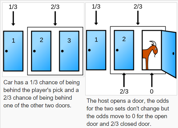
Suppose you are on a game show, and you have the choice of picking one of three doors: Behind one door is a car; behind the other doors, goats. You pick a door, let’s say door 1, and the host, who knows what’s behind the doors, opens another door, say door 3, which has a goat. The host then asks you: do you want to stick with your choice or choose another door?

Initially, for all three doors, the probability (P) of getting the car is the same $P = 1/3$. Now assume that the contestant chooses door 1, but it does not open. Next, the host opens the third door, which has a goat. Next, the host asks the contestant if he/she wants to switch the doors.
We can see that after the host opens door 3, the probability of the last two doors of having a car increases to 2/3. Now we know that the third door has a goat, and the likelihood of the second door having a car increases to 2/3. Hence, it is more advantageous to switch the doors. But let's test this with a Monte Carlo simulation.
# Game show test
# 1 - Car, 2 goats
doors = ['goat','goat','car']

# Empty lists to store probabilities
switch_win = []
stick_win = []

plt.axhline(y=0.66666, color='r',linestyle='-')
plt.axhline(y=0.33333,color='g',linestyle='-')
<matplotlib.lines.Line2D at 0x308b39990>

# Monte Carlo Game Show
def monte_carlo_game(n):
    '''
    Monte Carlo Simulation of a game show
    n is the number of simulations we wish to run
    '''

    #Calculating switch and stick wins
    switch_wins = 0
    stick_wins = 0

    for i in range(n):

        #Randomly placing the gar and goats
        random.shuffle(doors)

        #Contestant's choice
        k = random.randrange(2)

        # IF the contestant doesn't get the car
        if doors[k] != 'car':
            switch_wins += 1

        # If the contestant got the car:
        else:
            stick_wins += 1

        # Updating the list values
        switch_win.append(switch_wins/(i+1))
        stick_win.append(stick_wins/(i+1))

        # Plot the data
        plt.plot(switch_win)
        plt.plot(stick_win)

    # Print the probability values
    print('Winning probability if you always switch:',switch_win[-1])
    print('Winning probability if you always stick to your original choice:',stick_win[-1])
monte_carlo_game(1000)
Winning probability if you always switch: 0.667
Winning probability if you always stick to your original choice: 0.333

RocketSim
There are many tools you can use with Python and one such tool we can use is a toolbox called RocketPy. This tool allows us to load in different rocket motors, parachutes and other configurations. If you are interested in rocket simulation, I encourage you to check them out. For now, we will look at setting up a rocket and use a Monte Carlo simulation on the rocket setup.
Monte Carlo Simulations
This example wraps RocketPy's methods to run a Monte Carlo analysis and predict probability distributions of the rocket's landing point, apogee and other relevant information. The main output is a map very similar to the one below.

For this example we will look at the flight of Valetudo, one of the most famous rockets made by Projeto Jupiter. Valetudo has a diameter of $80$ mm and height of $2.4$ m. It was built for the first time to be launched at Latin American Space Challenge (LASC) 2019. Indeed, Valetudo came to be launched in 2019 on August 10th by 5:56 pm (local time), propelled by a class K motor called 'Keron', a solid motor completely designed and built by Projeto Jupiter. The rocket crossed the sky and reached an $860$ m apogee, descending safely by the drogue parachute called "Charmander" and landing with an 18.5 m/s terminal velocity.
Defining Analysis Parameters
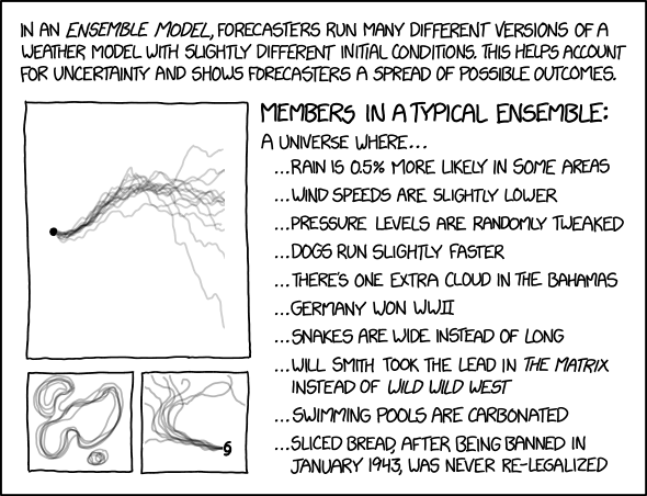
The analysis parameters are a collection of expected values (and their uncertainties, or standard deviation) that completely defines a rocket flight. As an assumption, the parameters which define the flight can behave in 3 different ways:
- the parameter is a completely known and has a constant value (i.e. number of fins)
- the parameter can assume certain discrete values with uniform distribution (i.e. the member of an ensemble forecast, which might be any integer from 0 to 9)
- the parameter is best represented by a normal (gaussian) distribution with a defined expected value and standard deviation
We implement this using a dictionary, where the key is the name of the parameter and the value is either a tuple or a list, depending on the behaviour of the parameter:
- if the parameter is know, its value is represented as a list with a single entry (i.e.
"number_of_fins: [4]") - if the parameter can assume certain discrete values with uniform distribution, its values are represented by a list of possible choices (i.e.
"member_of_ensemble_forecast: [0, 1, 2, 3, 4, 5, 6, 7, 8, 9]") - if the parameter is best represented by a normal (gaussian) distribution, its value is a tuple with the expected value and its standard deviation (i.e.
"rocket_mass": (100, 2), where 100 kg is the expected mass, with uncertainty of plus or minus 2 kg)
analysis_parameters = {
    # Mass Details
    "rocket_mass": (
        8.257,
        0.001,
    ),  # Rocket's dry mass (kg) and its uncertainty (standard deviation)
    # Propulsion Details - run help(SolidMotor) for more information
    "impulse": (1415.15, 35.3),  # Motor total impulse (N*s)
    "burn_time": (5.274, 1),  # Motor burn out time (s)
    "nozzle_radius": (21.642 / 1000, 0.5 / 1000),  # Motor's nozzle radius (m)
    "throat_radius": (8 / 1000, 0.5 / 1000),  # Motor's nozzle throat radius (m)
    "grain_separation": (
        6 / 1000,
        1 / 1000,
    ),  # Motor's grain separation (axial distance between two grains) (m)
    "grain_density": (1707, 50),  # Motor's grain density (kg/m^3)
    "grain_outer_radius": (21.4 / 1000, 0.375 / 1000),  # Motor's grain outer radius (m)
    "grain_initial_inner_radius": (
        9.65 / 1000,
        0.375 / 1000,
    ),  # Motor's grain inner radius (m)
    "grain_initial_height": (120 / 1000, 1 / 1000),  # Motor's grain height (m)
    # Aerodynamic Details - run help(Rocket) for more information
    "inertia_I": (
        3.675,
        0.03675,
    ),  # Rocket's inertia moment perpendicular to its axis (kg*m^2)
    "inertia_Z": (
        0.007,
        0.00007,
    ),  # Rocket's inertia moment relative to its axis (kg*m^2)
    "radius": (40.45 / 1000, 0.001),  # Rocket's radius (kg*m^2)
    "distance_rocket_nozzle": (
        -1.024,
        0.001,
    ),  # Distance between rocket's center of dry mass and nozzle exit plane (m) (negative)
    "distance_rocket_propellant": (
        -0.571,
        0.001,
    ),  # Distance between rocket's center of dry mass and and center of propellant mass (m) (negative)
    "power_off_drag": (
        0.9081 / 1.05,
        0.033,
    ),  # Multiplier for rocket's drag curve. Usually has a mean value of 1 and a uncertainty of 5% to 10%
    "power_on_drag": (
        0.9081 / 1.05,
        0.033,
    ),  # Multiplier for rocket's drag curve. Usually has a mean value of 1 and a uncertainty of 5% to 10%
    "nose_length": (0.274, 0.001),  # Rocket's nose cone length (m)
    "nose_distance_to_CM": (
        1.134,
        0.001,
    ),  # Axial distance between rocket's center of dry mass and nearest point in its nose cone (m)
    "fin_span": (0.077, 0.0005),  # Fin span (m)
    "fin_root_chord": (0.058, 0.0005),  # Fin root chord (m)
    "fin_tip_chord": (0.018, 0.0005),  # Fin tip chord (m)
    "fin_distance_to_CM": (
        -0.906,
        0.001,
    ),  # Axial distance between rocket's center of dry mass and nearest point in its fin (m)
    # Launch and Environment Details - run help(Environment) and help(Flight) for more information
    "inclination": (
        84.7,
        1,
    ),  # Launch rail inclination angle relative to the horizontal plane (degrees)
    "heading": (53, 2),  # Launch rail heading relative to north (degrees)
    "rail_length": (5.7, 0.0005),  # Launch rail length (m)
    "ensemble_member": list(range(10)),  # Members of the ensemble forecast to be used
    # Parachute Details - run help(Rocket) for more information
    "cd_s_drogue": (
        0.349 * 1.3,
        0.07,
    ),  # Drag coefficient times reference area for the drogue chute (m^2)
    "lag_rec": (
        1,
        0.5,
    ),  # Time delay between parachute ejection signal is detected and parachute is inflated (s)
    # Electronic Systems Details - run help(Rocket) for more information
    "lag_se": (
        0.73,
        0.16,
    ),  # Time delay between sensor signal is received and ejection signal is fired (s)
}
Creating a Flight Settings Generator
Now, we create a generator function which will yield all the necessary inputs for a single flight simulation. Each generated input will be randomly generated according to the analysis_parameters dicitionary set up above.
This is just a helper function to make the code clearer.
def flight_settings(analysis_parameters, total_number):
    i = 0
    while i < total_number:
        # Generate a flight setting
        flight_setting = {}
        for parameter_key, parameter_value in analysis_parameters.items():
            if type(parameter_value) is tuple:
                flight_setting[parameter_key] = normal(*parameter_value)
            else:
                flight_setting[parameter_key] = choice(parameter_value)

        # Skip if certain values are negative, which happens due to the normal curve but isnt realistic
        if flight_setting["lag_rec"] < 0 or flight_setting["lag_se"] < 0:
            continue

        # Update counter
        i += 1
        # Yield a flight setting
        yield flight_setting
Creating an Export Function
Monte Carlo analyses usually contain data from thousands or tens of thousands of simulations. They can easily take hours to run. Therefore, it is very important to save our outputs to a file during the analysis. This way, if something happens, we do not lose our progress.
These next functions take care of that. They export the simulation data to three different files:
dispersion_input_file: A file where each line is a json converted dictionary of flight setting inputs to run a single trajectory simulation;dispersion_output_file: A file where each line is a json converted dictionary containing the main outputs of a single simulation, such as apogee altitute and maximum velocity;dispersion_error_file: A file to store the inputs of simulations which raised errors. This can help us debug these simulations later on.
def export_flight_data(flight_setting, flight_data, exec_time):
    # Generate flight results
    flight_result = {
        "out_of_rail_time": flight_data.out_of_rail_time,
        "out_of_rail_velocity": flight_data.out_of_rail_velocity,
        "max_velocity": flight_data.speed.max,
        "apogee_time": flight_data.apogee_time,
        "apogee_altitude": flight_data.apogee - Env.elevation,
        "apogee_x": flight_data.apogee_x,
        "apogee_y": flight_data.apogee_y,
        "impact_time": flight_data.t_final,
        "impact_x": flight_data.x_impact,
        "impact_y": flight_data.y_impact,
        "impact_velocity": flight_data.impact_velocity,
        "initial_static_margin": flight_data.rocket.static_margin(0),
        "out_of_rail_static_margin": flight_data.rocket.static_margin(
            flight_data.out_of_rail_time
        ),
        "final_static_margin": flight_data.rocket.static_margin(
            flight_data.rocket.motor.burn_out_time
        ),
        "number_of_events": len(flight_data.parachute_events),
        "execution_time": exec_time,
    }

    # Take care of parachute results
    if len(flight_data.parachute_events) > 0:
        flight_result["drogue_triggerTime"] = flight_data.parachute_events[0][0]
        flight_result["drogue_inflated_time"] = (
            flight_data.parachute_events[0][0] + flight_data.parachute_events[0][1].lag
        )
        flight_result["drogue_inflated_velocity"] = flight_data.speed(
            flight_data.parachute_events[0][0] + flight_data.parachute_events[0][1].lag
        )
    else:
        flight_result["drogue_triggerTime"] = 0
        flight_result["drogue_inflated_time"] = 0
        flight_result["drogue_inflated_velocity"] = 0

    # Write flight setting and results to file
    dispersion_input_file.write(str(flight_setting) + "\n")
    dispersion_output_file.write(str(flight_result) + "\n")


def export_flight_error(flight_setting):
    dispersion_error_file.write(str(flight_setting) + "\n")
Simulating Each Flight Setting
Finally, we can start running some simulations! We start by defining the file name we want to use. Then, we specifiy how many simulations we would like to run by setting the number_of_simulations variable.
Each simulation takes a fair amount of time. While a good Monte Carlo simulation should have thousands of simulations, for now, we'll keep this to 100 in the interest of time. If you have some more time, you can always try running more. It is also good practice to run something in the order of 100 simulations first, to check for any possible errors in the code. Once we are confident that everything is working well, we increase the number of simulations to something in the range of 5000 to 50000.
We will loop throught all flight settings, creating the environment, rocket and motor classes with the data of the analysis parameters. For the power off and on drag and thrust curve user should have in hands the .csv (or .eng for comercial motor's thrust curve).
Note that we are using append instead of write for our files. This is often a better practice.
# Basic analysis info
filename = "dispersion_analysis_outputs/valetudo_rocket_v1"
number_of_simulations = 101

# Create data files for inputs, outputs and error logging
dispersion_error_file = open(str(filename) + ".disp_errors.txt", "a")
dispersion_input_file = open(str(filename) + ".disp_inputs.txt", "a")
dispersion_output_file = open(str(filename) + ".disp_outputs.txt", "a")

# Initialize counter and timer
i = 0

initial_wall_time = time()
initial_cpu_time = process_time()

# Define basic Environment object
Env = Environment(
    date=(2025, 4, 8, 21), latitude=-23.363611, longitude=-48.011389
)
Env.set_elevation(668)
Env.max_expected_height = 1500
Env.set_atmospheric_model(
    type="Ensemble",
    file="dispersion_analysis_inputs/LASC2019_reanalysis.nc",
    dictionary="ECMWF",
)

# Set up parachutes. This rocket, named Valetudo, only has a drogue chute.
def drogue_trigger(p, h, y):
    # Check if rocket is going down, i.e. if it has passed the apogee
    vertical_velocity = y[5]
    # Return true to activate parachute once the vertical velocity is negative
    return True if vertical_velocity < 0 else False


# Iterate over flight settings
out = display("Starting", display_id=True)
for setting in flight_settings(analysis_parameters, number_of_simulations):
    start_time = process_time()
    i += 1

    # Update environment object
    Env.select_ensemble_member(setting["ensemble_member"])

    # Create motor
    Keron = SolidMotor(
        thrust_source="dispersion_analysis_inputs/thrustCurve.csv",
        burn_time=5.274,
        reshape_thrust_curve=(setting["burn_time"], setting["impulse"]),
        nozzle_radius=setting["nozzle_radius"],
        throat_radius=setting["throat_radius"],
        grains_center_of_mass_position=setting["distance_rocket_propellant"],
        grain_number=6,
        grain_separation=setting["grain_separation"],
        grain_density=setting["grain_density"],
        grain_outer_radius=setting["grain_outer_radius"],
        grain_initial_inner_radius=setting["grain_initial_inner_radius"],
        grain_initial_height=setting["grain_initial_height"],
        interpolation_method="linear",
        nozzle_position=setting["distance_rocket_nozzle"],
        coordinate_system_orientation="nozzle_to_combustion_chamber",
        dry_mass=0,
        dry_inertia=(0, 0, 0),
        center_of_dry_mass_position=0
    )
    # Create rocket
    Valetudo = Rocket(
        radius=setting["radius"],
        mass=setting["rocket_mass"],
        inertia=(setting["inertia_I"],setting["inertia_I"],setting["inertia_Z"]),
        power_off_drag="dispersion_analysis_inputs/Cd_PowerOff.csv",
        power_on_drag="dispersion_analysis_inputs/Cd_PowerOn.csv",
        center_of_mass_without_motor=0,
        coordinate_system_orientation="tail_to_nose",
    )
    Valetudo.set_rail_buttons(0.224, -0.93, 30)

    Valetudo.add_motor(Keron, position=setting["distance_rocket_nozzle"])

    # Edit rocket drag
    Valetudo.power_off_drag *= setting["power_off_drag"]
    Valetudo.power_on_drag *= setting["power_on_drag"]
    # Add rocket nose, fins and tail
    NoseCone = Valetudo.add_nose(
        length=setting["nose_length"],
        kind="vonKarman",
        position=setting["nose_distance_to_CM"],
    )
    FinSet = Valetudo.add_trapezoidal_fins(
        n=3,
        span=setting["fin_span"],
        root_chord=setting["fin_root_chord"],
        tip_chord=setting["fin_tip_chord"],
        position=setting["fin_distance_to_CM"],
        cant_angle=0,
        airfoil=None,
    )
    # Add parachute
    Drogue = Valetudo.add_parachute(
        "Drogue",
        cd_s=setting["cd_s_drogue"],
        trigger=drogue_trigger,
        sampling_rate=105,
        lag=setting["lag_rec"] + setting["lag_se"],
        noise=(0, 8.3, 0.5),
    )

    # Run trajectory simulation
    try:
        test_flight = Flight(
            rocket=Valetudo,
            environment=Env,
            rail_length=setting["rail_length"],
            inclination=setting["inclination"],
            heading=setting["heading"],
            max_time=600,
        )
        export_flight_data(setting, test_flight, process_time() - start_time)
    except Exception as E:
        print(E)
        export_flight_error(setting)

    # Register time
    out.update(
        f"Curent iteration: {i:06d} | Average Time per Iteration: {(process_time() - initial_cpu_time)/i:2.6f} s"
    )

# Done

## Print and save total time
final_string = f"Completed {i} iterations successfully. Total CPU time: {process_time() - initial_cpu_time} s. Total wall time: {time() - initial_wall_time} s"
out.update(final_string)
dispersion_input_file.write(final_string + "\n")
dispersion_output_file.write(final_string + "\n")
dispersion_error_file.write(final_string + "\n")

## Close files
dispersion_input_file.close()
dispersion_output_file.close()
dispersion_error_file.close()
---------------------------------------------------------------------------
OSError                                   Traceback (most recent call last)
Cell In[13], line 22
     20 Env.set_elevation(668)
     21 Env.max_expected_height = 1500
---> 22 Env.set_atmospheric_model(
     23     type="Ensemble",
     24     file="dispersion_analysis_inputs/LASC2019_reanalysis.nc",
     25     dictionary="ECMWF",
     26 )
     28 # Set up parachutes. This rocket, named Valetudo, only has a drogue chute.
     29 def drogue_trigger(p, h, y):
     30     # Check if rocket is going down, i.e. if it has passed the apogee

File ~/anaconda3/lib/python3.11/site-packages/rocketpy/environment/environment.py:1283, in Environment.set_atmospheric_model(self, type, file, dictionary, pressure, temperature, wind_u, wind_v)
   1281         self.process_forecast_reanalysis(dataset, dictionary)
   1282     else:
-> 1283         self.process_ensemble(dataset, dictionary)
   1284 else:  # pragma: no cover
   1285     raise ValueError(f"Unknown model type '{type}'.")

File ~/anaconda3/lib/python3.11/site-packages/rocketpy/environment/environment.py:1974, in Environment.process_ensemble(self, file, dictionary)
   1972 # Read weather file
   1973 if isinstance(file, str):
-> 1974     data = netCDF4.Dataset(file)
   1975 else:
   1976     data = file

File src/netCDF4/_netCDF4.pyx:2521, in netCDF4._netCDF4.Dataset.__init__()

File src/netCDF4/_netCDF4.pyx:2158, in netCDF4._netCDF4._ensure_nc_success()

OSError: [Errno -51] NetCDF: Unknown file format: 'dispersion_analysis_inputs/LASC2019_reanalysis.nc'
Post-processing Monte Carlo Dispersion Results
Now that we have finish running thousands of simulations, it is time to process the results and get some nice graphs out of them! Importing Dispersion Analysis Saved Data
We start by loading the file which stores the outputs.
filename = "dispersion_analysis_outputs/valetudo_rocket_v1"

# Initialize variable to store all results
dispersion_general_results = []

dispersion_results = {
    "out_of_rail_time": [],
    "out_of_rail_velocity": [],
    "apogee_time": [],
    "apogee_altitude": [],
    "apogee_x": [],
    "apogee_y": [],
    "impact_time": [],
    "impact_x": [],
    "impact_y": [],
    "impact_velocity": [],
    "initial_static_margin": [],
    "out_of_rail_static_margin": [],
    "final_static_margin": [],
    "number_of_events": [],
    "max_velocity": [],
    "drogue_triggerTime": [],
    "drogue_inflated_time": [],
    "drogue_inflated_velocity": [],
    "execution_time": [],
}

# Get all dispersion results
# Get file
dispersion_output_file = open(str(filename) + ".disp_outputs.txt", "r+")

# Read each line of the file and convert to dict
for line in dispersion_output_file:
    # Skip comments lines
    if line[0] != "{":
        continue
    # Eval results and store them
    flight_result = eval(line)
    dispersion_general_results.append(flight_result)
    for parameter_key, parameter_value in flight_result.items():
        dispersion_results[parameter_key].append(parameter_value)

# Close data file
dispersion_output_file.close()

# Print number of flights simulated
N = len(dispersion_general_results)
print("Number of simulations: ", N)
Number of simulations: 301
Mapping the results
There is a lot of information we can gather from this analysis, but for now, let's look at the results in terms of where we think the rocket will hit apogee and where it will land.
# Import background map
img = imageio.v2.imread("dispersion_analysis_inputs/Valetudo_basemap_final.jpg")

# Retrieve dispersion data por apogee and impact XY position
apogee_x = np.array(dispersion_results["apogee_x"])
apogee_y = np.array(dispersion_results["apogee_y"])
impact_x = np.array(dispersion_results["impact_x"])
impact_y = np.array(dispersion_results["impact_y"])

# Define function to calculate eigen values
def eigsorted(cov):
    vals, vecs = np.linalg.eigh(cov)
    order = vals.argsort()[::-1]
    return vals[order], vecs[:, order]


# Create plot figure
plt.figure(num=None, figsize=(8, 6), dpi=150, facecolor="w", edgecolor="k")
ax = plt.subplot(111)

# Calculate error ellipses for impact
impactCov = np.cov(impact_x, impact_y)
impactVals, impactVecs = eigsorted(impactCov)
impactTheta = np.degrees(np.arctan2(*impactVecs[:, 0][::-1]))
impactW, impactH = 2 * np.sqrt(impactVals)

# Draw error ellipses for impact
impact_ellipses = []
for j in [1, 2, 3]:
    impactEll = Ellipse(
        xy=(np.mean(impact_x), np.mean(impact_y)),
        width=impactW * j,
        height=impactH * j,
        angle=impactTheta,
        color="black",
    )
    impactEll.set_facecolor((0, 0, 1, 0.2))
    impact_ellipses.append(impactEll)
    ax.add_artist(impactEll)

# Calculate error ellipses for apogee
apogeeCov = np.cov(apogee_x, apogee_y)
apogeeVals, apogeeVecs = eigsorted(apogeeCov)
apogeeTheta = np.degrees(np.arctan2(*apogeeVecs[:, 0][::-1]))
apogeeW, apogeeH = 2 * np.sqrt(apogeeVals)

# Draw error ellipses for apogee
for j in [1, 2, 3]:
    apogeeEll = Ellipse(
        xy=(np.mean(apogee_x), np.mean(apogee_y)),
        width=apogeeW * j,
        height=apogeeH * j,
        angle=apogeeTheta,
        color="black",
    )
    apogeeEll.set_facecolor((0, 1, 0, 0.2))
    ax.add_artist(apogeeEll)

# Draw launch point
plt.scatter(0, 0, s=30, marker="*", color="black", label="Launch Point")
# Draw apogee points
plt.scatter(apogee_x, apogee_y, s=5, marker="^", color="green", label="Simulated Apogee")
# Draw impact points
plt.scatter(
    impact_x, impact_y, s=5, marker="v", color="blue", label="Simulated Landing Point"
)
# Draw real landing point
plt.scatter(
    411.89, -61.07, s=20, marker="X", color="red", label="Measured Landing Point"
)

plt.legend()

# Add title and labels to plot
ax.set_title(
    "1$\sigma$, 2$\sigma$ and 3$\sigma$ Dispersion Ellipses: Apogee and Lading Points"
)
ax.set_ylabel("North (m)")
ax.set_xlabel("East (m)")

# Add background image to plot
# You can translate the basemap by changing dx and dy (in meters)
dx = 0
dy = 0
plt.imshow(img, zorder=0, extent=[-1000 - dx, 1000 - dx, -1000 - dy, 1000 - dy])
plt.axhline(0, color="black", linewidth=0.5)
plt.axvline(0, color="black", linewidth=0.5)
plt.xlim(-100, 700)
plt.ylim(-300, 300)

# Save plot and show result
plt.savefig(str(filename) + ".pdf", bbox_inches="tight", pad_inches=0)
plt.show()

Questions?
